Optimal padding for convolution with the FFT
The Fast Fourier Transform (FFT) is fundamental to digital signal processing as it enables the (circular) convolution of two signals of length \(n\) to be computed in \(\mathcal{O}(n \log n)\) time. Different algorithms must be used for different \(n\) in order to achieve this asymptotic bound (see this paper on the design of FFTW for more details). Non-periodic convolutions can be computed by simply taking a subset of the output elements. However, in this scenario, it might be possible to use a faster algorithm by considering larger circular convolutions than necessary, padding the signals with arbitrary values. This article will investigate how to find a somewhat-optimal size.
Cooley-Tukey algorithm
This is perhaps the most well-known algorithm for computing the FFT. It notes that if the signal length \(n\) can be factored \(n = n_{1} n_{2}\), then the transform of length \(n\) can be computed using \(n_{1}\) transforms of length \(n_{2}\) and \(n_{2}\) transforms of length \(n_{1}\). The cost of computing the FFT is thus
\[f(n) = \begin{cases} n_{1} f(n_{2}) + n_{2} f(n_{1}), & \text{if $n = n_{1} n_{2}$,} \\ n^{2}, & \text{if $n$ is prime.} \end{cases}\]Let the prime factorisation of \(n\) be \(n = k_{1} k_{2} \cdots k_{m}\). Then the cost of the transform is
\[\begin{align} f(n) & = (k_{2} \cdots k_{m}) k_{1}^{2} + k_{1} f(k_{2} \cdots k_{m}) \\ & = n k_{1} + k_{1} \left[ (k_{3} \cdots k_{m}) k_{2}^{2} + k_{2} f(k_{3} \cdots k_{m}) \right] \\ & = n (k_{1} + k_{2}) + k_{1} k_{2} f(k_{3} \cdots k_{m}) \\ & = \cdots \\ & = n ({\textstyle \sum_{i} k_{i}}) . \end{align}\]We can thus see that if \(n = k^{m}\) with \(k\) some small constant, then \(f(n) = n k \log_{k} n\) is \(\mathcal{O}(n \log n)\). However, if \(n\) is prime then the complexity will still be \(\mathcal{O}(n^2)\), and if \(n\) has large prime factors then the algorithm will be several times slower than with small.
Next power of a few small primes
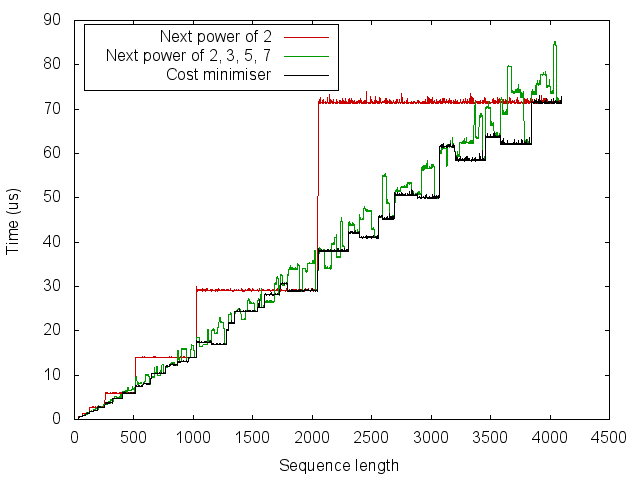
A simple heuristic is therefore to round the length up to the next power of a few small primes. In the following experiment, we compare computing the FFT of size \(n\) to the next power of 2 as well as to the next number of the form \(2^{a} 3^{b} 5^{c} 7^{d}\).
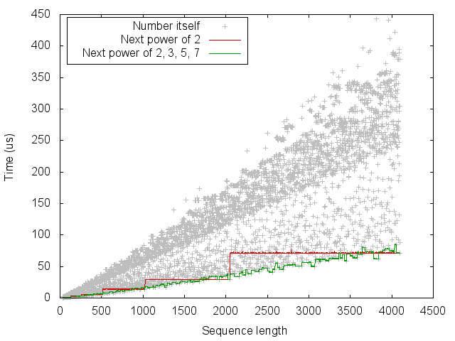
From this we can see that the simple heuristic of rounding up to the next power of 2 gives a big improvement for some sizes, but can be up to twice as slow. Using the next power of 2, 3, 5 and 7 is often but not always better than the next power of 2. It should be possible to achieve the staircase-like curve which lower-bounds this set of points. However, we would like to do so without measuring the running time for every size.
The first thing that I tried was to find the number \(m = 2^{a} 3^{b} 5^{c} 7^{d} \ge n\) which minimises
\[f(m) = g(a, b, c, d) = (2^{a} 3^{b} 5^{c} 7^{d}) (2a+3b+5c+7d).\]This was found using depth-first search in a tree whose edges each correspond to incrementing one of \(\{a, b, c, d\}\).
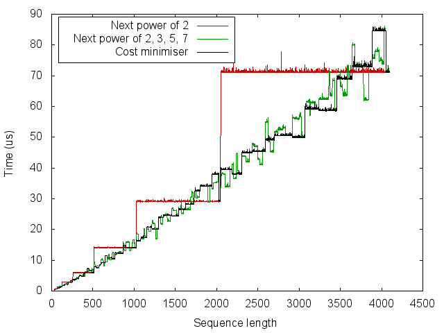
The result is not resounding. Delving into the FFTW paper, the authors mention that they use highly optimised “codelets” for sizes 2, …, 32, 64. Resorting to (mild) hacks, we can incorporate this into the cost function by decomposing \(a = \min(a, \tau) + \max(0, a-\tau)\), where \(\tau = 6\) to consider a maximum codelet size of \(64 = 2^6\). We then introduce a relative acceleration \(r \ge 1\) which applies to the first \(\tau\) powers of 2. The modified cost function is
\[g'(a, b, c, d) = (2^{a} 3^{b} 5^{c} 7^{d}) \left(2\left[\min(a, \tau) / r + \max(0, a-\tau)\right]+3b+5c+7d \right)\]The results using \(\tau = 6\) and \(r = 2\) are not perfect but better.