General trajectory prior for non-rigid reconstruction
Consider a 3D object deforming non-rigidly over time, for example:
The object is observed by a single moving camera. We want to recover the 3D structure from these 2D projection correspondences.
Let’s assume that the camera motion relative to the background can be recovered using rigid structure from motion. With known cameras, each 2D projection of a point defines a 2x3 linear system of equations for its 3D position in that frame.
\[\mathbf{u}_{t} = \mathbf{Q}_{t} \mathbf{x}_{t}\]The 1D nullspace of this system corresponds geometrically to a ray departing from the camera centre.
This means that using only projection constraints, there are infinite solutions for each point in each frame (anywhere along those rays). However, we know intuitively that points should not jump around arbitrarily from frame to frame. Assuming that the points have mass, their motion should be smooth (since they must be accelerated by a finite force). This notion was leveraged by Akhter et al (2008), who required that the trajectory of each point be expressed as a sum of low frequency sinusoids i.e. lie on the subspace of a truncated DCT basis.
Stacking the equations for the observation of a point in all F frames yields a 2Fx3F system.
\[\begin{bmatrix} \mathbf{u}_{1} \\ \vdots \\ \mathbf{u}_{F} \end{bmatrix} = \begin{bmatrix} \mathbf{Q}_{1} \\ & \ddots \\ & & \mathbf{Q}_{F} \end{bmatrix} \begin{bmatrix} \mathbf{x}_{1} \\ \vdots \\ \mathbf{x}_{F} \end{bmatrix}, \qquad \mathbf{u} = \mathbf{Q} \mathbf{x}\]Introducing a K-dimensional DCT basis for the x, y and z components of the trajectory, the system of equations becomes 2Fx3K.
\[\mathbf{x}^{*} = \mathbf{\Theta} \boldsymbol{\beta}^{*}, \qquad \boldsymbol{\beta}^{*} = \arg \min_{\boldsymbol{\beta}} \; \left\lVert \mathbf{u} - \mathbf{Q} \mathbf{\Theta} \boldsymbol{\beta} \right\rVert^{2}\]While this problem is not necessarily underconstrained if 3K ≤ 2F, Park et al (2010) found that significant camera motion was also required to obtain an accurate reconstruction, establishing the notion of reconstructability. The following figure shows reconstruction error versus camera speed for varying basis size K, generated from a synthetic experiment in which human motion capture sequences (of 100 frames) are observed by an orbiting camera.
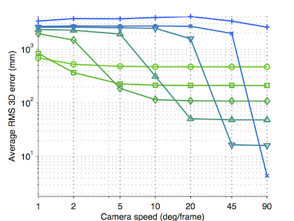

The key observation here is that faster moving cameras enable more accurate reconstruction. However, you have to choose the basis size correctly or else you will either run out of capacity to represent the points’ motion (to the right) or revert to an ill-posed problem (to the left).
Park et al defined a measure of reconstructability depending on how well the camera trajectory was represented by the basis, since, if the camera centre lies on the basis, its trajectory is a trivial solution. We defined a new measure based on a theoretical bound on the reconstruction error. Our measure does not depend on the camera centre, rather, it incorporates the condition number of the linear system of equations, the ratio of the largest eigenvalue to the smallest.
The implications of this become clearer when we alternatively consider minimising the distance of the trajectory from the DCT subspace, subject to the 2D projections being exactly satisfied.
\[\mathbf{x}^{*} = \arg \min_{\mathbf{x}} \; \left\lVert \left(\mathbf{I} - \mathbf{\Theta} \mathbf{\Theta}^{T}\right) \mathbf{x} \right\rVert^{2} \; \text{s.t.} \; \mathbf{u} = \mathbf{Q} \mathbf{x}\]Since the DCT matrix is rank 3K, the orthogonal projection matrix in the objective will have a nullspace of dimension 3K. When we reduce K, we reduce the size of this nullspace and therefore reduce the likelihood of having a poorly-conditioned system. Consider the more general form
\[\mathbf{x}^{*} = \arg \min_{\mathbf{x}} \; \mathbf{x}^{T} \mathbf{M} \mathbf{x} \; \text{s.t.} \; \mathbf{u} = \mathbf{Q} \mathbf{x}.\]We propose that the conditioning problem can be mostly avoided by choosing
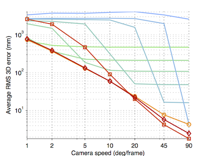
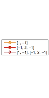
\[\mathbf{M} = \mathbf{G}^{T} \mathbf{G}, \qquad \mathbf{G} \mathbf{x} = \mathbf{g} * \mathbf{x}\]where multiplication by the matrix G is equivalent to convolution with the filter g (note that we define vector convolution to operate independently in x, y, z.) We typically choose simple finite difference filters: some combination of (-1, 1) and (-1, 2, -1). If the filter has support m, then the matrix M has a nullspace of size 3(m-1), since we only compute the convolution with parts of the signal where the two inputs overlap completely (i.e. “valid” mode in Matlab’s conv() function).
Using these “trajectory filters,” we are able to achieve 3D error at the limit of reconstructability without having to choose the basis size K.
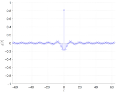
The reason that this works becomes evident examining the eigenspectra of the DCT matrix (left) versus the first-difference (middle) and second-difference (right) filters. The filters do not have the many zero eigenvalues which cause the system to become poorly conditioned.
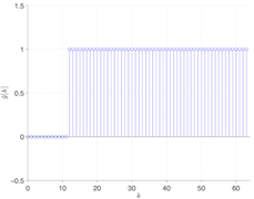
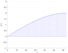
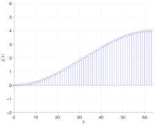
A nice twist here is that the Discrete Cosine Transform diagonalises symmetric convolution in an analogous way to the Fourier transform diagonalising periodic convolution, so the eigenspectra above are actually the DCT transform of each filter. This means we can enforce the filters as a weighting in the DCT domain, although in practice it is usually more efficient to work in the time domain because the systems are sparse. This also makes it possible to reveal the filter which is equivalent to using a particular truncation of the DCT basis.
The final results from our example are shown below. Red points denote the output and black the ground truth.
Code
I’ve tried to provide sufficient code and data to reproduce the figures in the paper. It’s all Matlab. Never tested with GNU Octave. This code is provided for free use, no warranty whatsoever.
Run setup.m to set the path as required.
The main figures (reconstruction error versus camera speed) can be generated by running solver_experiment.m. Note that averaging these experiments over as many trials as we did probably requires a compute cluster or significant hours. You can reduce the number of trials though, for slightly less-smooth curves.
This experiment depends on Honglak Lee et al’s implementation of their feature-sign search algorithm for the comparison to sparse coding methods. Ensure that l1ls_featuresign.m is found in src/lee-2006/.
I’m also providing the exact 100-frame mocap sequences from the CMU Motion Capture Database which we used. Thanks to Mark Cox for converting them to point clouds. Put this file in data/ before running solver_experiment.m.
The actual reconstruction code is super simple and happens in reconstruct_filters.m and reconstruct_linear.m. The linear systems for projection constraints are constructed in trajectory_projection_equations.m, projection_equation.m and independent_to_full.m.
The videos on this webpage are generated by running filters_demo.m. To save the movies you’ll need the ImageMagick convert utility and ffmpeg (both free).
The qualitative examples from real photos are generated by running real_scene_demo.m. To do this, you’ll need to download the “Real scene” data from Hyun Soo Park’s project page and unzip it to data/RealSceneData/. I’ve also re-distributed two small functions from his code in src/park-2010/.