Sampling smooth paths
Sometimes it’s useful to generate random smooth paths that hang around the origin. The simplest way to obtain a random path is to generate a random walk where each step is independent and normally distributed. To make the path smooth, we have a couple of options: (1) we could smooth the path with a low-pass filter, or (2) we could integrate the random walk again such that the second derivative is normally distributed rather than the first derivative. However, one problem with these approaches is that the paths might stray arbitrarily far from the origin. Here’s a simple technique that I use to generate smooth paths that don’t stray too far.
Let’s consider the problem of sampling a path of length $N$ in one dimension. We can always sample multiple independent paths to obtain a multi-dimensional path. The idea is simply to sample from a Gaussian distribution with precision matrix (inverse covariance matrix)
\[\Lambda = I + \alpha \Lambda_{1} + \beta \Lambda_{2}\]where $\Lambda_1 = D_1^T D_1$ and $\Lambda_2 = D_2^T D_2$ and $D_{i}$ is a finite difference operator of order $i$.
\[D_1 = \begin{bmatrix} -1 & 1 \\ & -1 & 1 \\ && \ddots & \ddots \\ &&& -1 & 1 \end{bmatrix}\] \[D_2 = \begin{bmatrix} -1 & 2 & -1 \\ & -1 & 2 & -1 \\ && \ddots & \ddots & \ddots \\ &&& -1 & 2 & -1 \end{bmatrix}\]Then finite difference matrix $D_i$ has shape $(N - i) \times N$.
To sample from the distribution $\mathcal{N}(0, \Lambda^{-1})$, we need a matrix $A$ such that $A A^{T} = \Lambda^{-1}$. This can be obtained by computing an eigendecomposition $\Lambda = V D V^T$ and setting $A = V D^{-\frac{1}{2}}$. To obtain a path, we then take $x = A \epsilon$ where $\epsilon$ is drawn from a unit normal distribution.
Efficient technique
However, the above approach requires us to compute a factorization of a large (admittedly sparse) matrix. This can be avoided if we are willing to instead consider sampling periodic smooth paths. If we assume the paths to be periodic, then the finite difference matrices will be square and circulant.
\[D_1 = \begin{bmatrix} -1 & 1 \\ & -1 & 1 \\ && \ddots & \ddots \\ &&& -1 & 1 \\ 1 &&&& -1 \end{bmatrix}\]Circulant matrices can be diagonalized using the Discrete Fourier Transform. For engineers like me, this diagonalization is hiding in the familiar convolution identity. Let $Y$ denote the matrix which corresponds to circular convolution with a signal $y$.
\[Y x = y \star x\] \[F Y x = F (y \star x) = (F y) \odot (F x) = \operatorname{diag}(F y) F x\] \[Y x = F^{-1} \operatorname{diag}(F y) F x \qquad \forall x\] \[Y = F^{-1} \operatorname{diag}(F y) F\]Here the $F$ matrix computes the DFT in the same way as the function fft() in numpy.
Note that this matrix is not unitary but instead satisfies
For convenience, let us define $U = \frac{1}{\sqrt{N}} F$ so that $U^{-1} = U^{\ast}$ and the diagonalization can be expressed:
\[Y = (\sqrt{N} U)^{-1} \operatorname{diag}(F y) (\sqrt{N} U) = U^{\ast} \operatorname{diag}(F y) U\]Now we can use this to diagonalize the finite difference matrix:
\[D_{1} = U^{\ast} \operatorname{diag}(F d_{1}) U\]where $d_{1} = (-1, 1, 0, \dots, 0)$. The Gram matrix becomes
\[D_{1}^{T} D_{1} = D_{1}^{\ast} D_{1} = U^{\ast} \operatorname{diag}(F d_{1})^{\ast} U U^{\ast} \operatorname{diag}(F d_{1}) U = U^{\ast} \operatorname{diag}(\lvert F d_{1} \rvert^{2}) U\]Finally, the entire precision matrix $\Lambda$ can therefore be diagonalized $\Lambda = U^{\ast} \operatorname{diag}(\lambda) U$ where
\[\lambda = \lvert F \delta \rvert^{2} + \alpha \lvert F d_{1} \rvert^{2} + \beta \lvert F d_{2} \rvert^{2}\]Note that $F \delta = 1$. Incidentally, since $d_2 = d_1 \star d_1$, we see that $F d_{2} = (F d_{1})^2$ and therefore $\lvert F d_{2} \rvert^2 = \lvert F d_{1} \rvert^4$.
Therefore, to sample from the distribution $\mathcal{N}(0, \Lambda^{-1})$, it seems that we could use the matrix
\[A = U^{\ast} \operatorname{diag}(\lambda^{-\frac{1}{2}})\]But wait, something seems wrong here. The precision matrix $\Lambda$ is symmetric positive-definite and yet the eigenvectors in $U$ are complex? In order to obtain samples $x = A \epsilon$, we need a real factorization $\Sigma = A A^{T}$.
Real diagonalization
What’s happened here is that some eigenvalues occur twice and therefore the eigenvectors are not unique: we can take any (complex) rotation of two eigenvectors with the same eigenvalue and they are still unit-norm eigenvectors of the same matrix. It should be possible to mix these eigenvectors in a way that makes them real.
Recall that the Fourier transform of a real-valued signal has conjugate symmetry. We can immediately observe that the transform $\lambda$ possesses real symmetry since it is obtained from the magnitude of a transform with conjugate symmetry. Therefore the identical eigenvalues occur at $\lambda[k]$ and $\lambda[N - k]$.
From the diagonalization $\Lambda = U^{\ast} \operatorname{diag}(\lambda) U$ we can see that the eigenvalues correspond to rows of $U$. Happily, the rows of $U$ possess conjugate symmetry. Recall from the definition of the DFT matrix $F$ (which is related to the unitary matrix $U$ by a scalar) that element $s, t$ of the DFT matrix is $F_{s, t} = \omega_{N}^{s t}$ where $\omega_{N} = \exp(i 2 \pi / N)$. Using the fact that $\omega_{N}^{n} = \omega_{N}^{n \bmod N}$ we see the symmetry in the rows of $F$:
\[\left\{ \begin{aligned} F_{s, t} & = \omega_{N}^{s t} \\ F_{N - s, t} & = \omega_{N}^{(N - s) t} = \omega_{N}^{-s t} = \bar{F}_{s, t} \end{aligned} \right.\]There are two special cases. For $s = 0$, we have $F_{s, t} = \omega_{N}^{0} = 1$, which is already real. For $s = N / 2$ (only when $N$ is even), we have $F_{s, t} = \omega_{N}^{(N/2) t} = (-1)^{t}$, which is also already real.
Therefore we propose to introduce an orthonormal complex matrix $Q$ such that $V = Q U$ is real and therefore $V^{T} = V^{\ast} = V^{-1}$. Let $U_{k}$ denote row $k$ of the matrix $U$. Let $Q_{k}$ denote the submatrix of elements $\{k, N - k\} \times \{k, N - k\}$ of the matrix $Q$. If we let $Q_{k}$ take the form
\[Q_{k} = \begin{bmatrix} \alpha & \alpha \\ -i \beta & i \beta \end{bmatrix}\]then we see that
\[\begin{align} Q_{k} \begin{bmatrix} U_{k} \\ U_{N - k} \end{bmatrix} & = \begin{bmatrix} \alpha & \alpha \\ -i \beta & i \beta \end{bmatrix} \begin{bmatrix} U_{k} \\ \bar{U}_{k} \end{bmatrix} \\ & = \begin{bmatrix} \alpha 2 \operatorname{Re}\{U_{k}\} \\ \beta 2 \operatorname{Im}\{U_{k}\} \end{bmatrix} \end{align}\]which is real. To preserve orthogonality, we choose $\alpha = \beta = \frac{1}{\sqrt{2}}$. This will have no effect on the eigenvalues since
\[Q_{k}^{\ast} (\lambda_k I_{2}) Q_{k} = \lambda_k Q_{k}^{\ast} Q_{k} = \lambda_k I_2\]Overall our $Q$ matrix takes the form
\[Q = \begin{bmatrix} 1 \\ & \frac{1}{\sqrt{2}} &&&&&& \frac{1}{\sqrt{2}} \\ && \frac{1}{\sqrt{2}} &&&& \frac{1}{\sqrt{2}} \\ &&& \ddots && \ddots \\ &&&& (1) \\ &&& \ddots && \ddots \\ && -i \frac{1}{\sqrt{2}} &&&& i \frac{1}{\sqrt{2}} \\ & -i \frac{1}{\sqrt{2}} &&&&&& i \frac{1}{\sqrt{2}} \end{bmatrix}\]Finally, we have our real $A = U^{\ast} Q^{\ast} \operatorname{diag}(\lambda^{-\frac{1}{2}})$. Since $U^{\ast} = \frac{1}{\sqrt{N}} F^{\ast} = \sqrt{N} F^{-1}$, samples can be obtained
\[x = \sqrt{N} \cdot \operatorname{ifft}(Q^{\ast}(\lambda^{-\frac{1}{2}} \circ \epsilon))\]Note that the operation $Q^{\ast}$ can be implemented as follows
\[(Q^{\ast} h)[k] = \begin{cases} h[k], & k = 0 \\ \frac{1}{\sqrt{2}} (h[k] + i h[N - k]), & 0 < k < N / 2 \\ h[k], & k = N / 2 \\ \frac{1}{\sqrt{2}} (h[k] - i h[N - k]), & N / 2 < k \end{cases}\]When $h$ is real and symmetric (as above), this is equivalent to
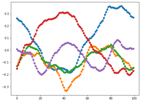
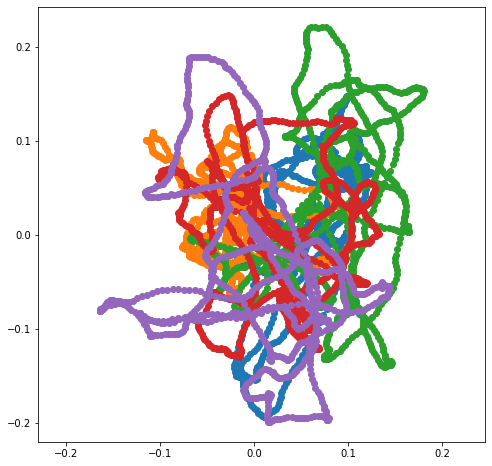
\[(Q^{\ast} h)[k] = \begin{cases} h[k], & k = 0 \\ \frac{1}{\sqrt{2}} (1 + i) h[k], & 0 < k < N / 2 \\ h[k], & k = N / 2 \\ \frac{1}{\sqrt{2}} (1 - i) h[k], & N / 2 < k \end{cases}\]Here are a few smaples from this distribution. I often use $\alpha = 0$ and $\beta \in [10^3, 10^6]$. Note that, since the paths are constrained to be periodic, shorter paths may be tightly clustered.
Of course, if we want to generate non-periodic paths, we can generate a periodic path of a larger size and then truncate it.